Automated Canvas Quiz Generation with R exams
Introduction
Manual quiz entry in Canvas is tedious and prone to error. In this approach, the problem and its structure are designed by the instructor to ensure pedagogical alignment, while the data generation and Canvas integration are streamlined with R for massive scalability.
Motivation: Accountability Through Uniqueness
I design realistic data-driven business challenges for individual assignments. By ensuring every student has a unique “correct” answer based on their specific dataset, I can encourage peer collaboration while strictly enforcing individual accountability. Students can discuss methods and formulas, but they cannot simply ‘borrow’ answers.
Project Architecture: Templates vs. Compilation
Before diving into the code, it is important to understand how the R/exams ecosystem is structured. A typical project consists of two distinct types of files:
- Question Templates (
Q1.Rmd,Q2.Rmd, etc.): These are standalone files that contain the logic for a single question. Each file handles its own data generation, question text, and solution mapping. - The Compilation Script (
compile.Rmd): This is the “manager” script. It calls the question templates, specifies how many randomized versions to create (e.g., $n=100$), and handles the final export to Canvas.
In a real-world scenario, your Canvas quiz will likely contain multiple questions. However, to keep this guide focused, we will demonstrate the end-to-end workflow using a single, Linear Regression Challenge.
1. The Data Generation Chunk
The data generation chunk is the “brain” of the question. Because it handles everything from raw data fetching to answer key generation, we will build it piece by piece. Note that in your final .Rmd file, all these snippets belong inside a single ````{r}` block.
Part A: Fetching and Cleaning Real-World Data
We lead with the worldfootballR package to pull live performance data. This ensures our students are working with realistic, timely scenarios.
library(exams)
library(data.table)
library(worldfootballR)
library(stringr)

# Fetching advanced passing and possession stats for the 2023/24 season
passing <- load_fb_big5_advanced_season_stats(
  season_end_year = 2024, stat_type = "passing", team_or_player = "player"
) |> data.table()

poss <- load_fb_big5_advanced_season_stats(
  season_end_year = 2024, stat_type = "possession", team_or_player = "player"
) |> data.table()

# Merge and clean position labels
soccer_data <- cbind(
  passing[, .(Club = Squad, Player, Position = Pos, Mins_Per_90,
              Completed_Passes = Cmp_Total / Mins_Per_90)],
  poss[, .(Touches = Touches_Touches / Mins_Per_90)]
)

soccer_data <- soccer_data[Mins_Per_90 > 5 & Position != "GK"]
soccer_data[, Position := str_split_fixed(Position, ",", 3)[, 1]]
Part B: Injecting Individualized Noise
This is the most critical step for academic integrity. By adding a unique “jitter” to the data for every version, we ensure that while the process is the same for every student, the numerical results are unique.
# Every time this template 'knits', the noise changes
soccer_data[Position == "FW", Completed_Passes := Completed_Passes + runif(.N, -0.9, 0.3)]
soccer_data[Completed_Passes < 0, Completed_Passes := 0]

# Build the 'Ground Truth' Model that the student must find
soccer_data[, Position := forcats::fct_relevel(factor(Position), "FW")]
my_reg <- lm(Completed_Passes ~ Position + Touches, soccer_data)
coef_table <- summary(my_reg)$coefficients
Part C: Automating Data Delivery (OneDrive)
Since students need unique datasets, we must host them somewhere accessible. Using the Microsoft365R package, we can automate the process of uploading each Excel file to OneDrive and generating a sharing link.
library(Microsoft365R)
library(openxlsx)

od <- get_personal_onedrive()

# Save the unique dataset to a temporary Excel file
temp_file_path <- tempfile(fileext = ".xlsx")
write.xlsx(soccer_data, temp_file_path, colNames = TRUE, rowNames = FALSE)

# Generate a unique destination path
v_num <- nrow(od$list_items("teaching_assets")) + 1
dest_file <- glue("teaching_assets/dataset_{v_num}.xlsx")

# Upload and generate a 'view' link
od$upload_file(src = temp_file_path, dest = dest_file)
download_url <- od$get_item(dest_file)$create_share_link("view")
Part D: Generating Answers and Solution Mapping
Finally, we programmatically create the multiple-choice options. In R/exams, we typically structure each part as a character vector where the first element is the correct answer, followed by several distractors. This order is later randomized in Canvas.
library(glue)

# Part 1: Interpretations for Touches
# We use glue to insert the student's unique coefficient into the text
coef <- abs(signif(coef_table["Touches", "Estimate"], 2))
part1 <- c(
  glue("For every additional touch, expected passes increase by {coef}."),
  glue("For every completed pass, expected ball touches increase by {coef}."),
  glue("If a player has zero touches, expected passes are {coef}.")
)

# Part 2: Categorical Comparison (MD vs FW)
coef <- abs(signif(coef_table["PositionMF", "Estimate"], 3))
part2 <- c(
  glue("Holding Touches constant, a Midfielder completes more passes than a Forward by {coef}."),
  glue("Holding Touches constant, a Midfielder completes fewer passes than a Forward by {coef}."),
  glue("A Midfielder's total number of completed passes is equal to {coef}.")
)
For more complex evaluations, like statistical significance, we can use conditional logic to ensure the “Correct” answer is always placed at the start of the vector.
# Part 3: Statistical Significance Logic
p_md <- coef_table["PositionMF", "Pr(>|t|)"]
p_df <- coef_table["PositionDF", "Pr(>|t|)"]

options <- c(
  "Both Midfielder and Defender are significant.",
  "Neither coefficient is significant.",
  "Midfielder is significant, but Defender is not.",
  "Defender is significant, but Midfielder is not."
)

# Logical mapping to find the correct index based on unique p-values
correct_idx <- ifelse(p_md < 0.05, ifelse(p_df < 0.05, 1, 3), ifelse(p_df < 0.05, 4, 2))
part3 <- c(options[correct_idx], options[-correct_idx])

# Part 4: Numerical Prediction with Random Distractors
pred_data <- soccer_data[1, ] # Simplified prediction data
pred_data[, `:=`(Position = "MF", Touches = 90)]
correct_val <- predict(my_reg, pred_data)
part4 <- c(
  correct_val,
  correct_val + sample(c(-5, 5, 10, -10), size = 3)
) |> round(2)
Part E: The Solution String
Because the correct answer is always at index 1 for every part, our solution mapping for Canvas becomes a simple repeated string of binary indicators.
# Generate the solution string (e.g., "100|100|1000|1000")
# 1 indicates the first element is the correct one, 0s are distractors
sols <- sapply(paste0("part", 1:4), function(x){
  ans_len <- length(get(x))
  paste0("1", paste0(rep("0", ans_len - 1), collapse = ""))
})
solution_list <- paste(sols, collapse = "|")
2. The Question Section
The Question section uses Markdown to present the case study narrative. We leverage R inline code to customize the experience for each student.
Notice the Markdown table at the end of the question block. This table is not just for formatting text; it acts as a layout grid for the interactive quiz elements. The ##ANSWER## tags (known as “Cloze” placeholders) tell Canvas exactly where to embed the dropdown menus or numerical input boxes that students will interact with.
Question
========
You are a data analyst for San Diego FC (SDFC), a Major League Soccer (MLS) team that began play in
2025. Your focus is international scouting, particularly from European leagues, to identify
potential transfer targets.
To aid in this process, you will build a regression model using data exclusively from players in
Europe's top five leagues. The goal is to use this European benchmark model to project a player's
passing ability, helping the team assess if a potential signing's style will translate well to
SDFC's system.
The model will predict a player's completed passes per game based on the average number of times the
player makes contact with the ball and their playing position.
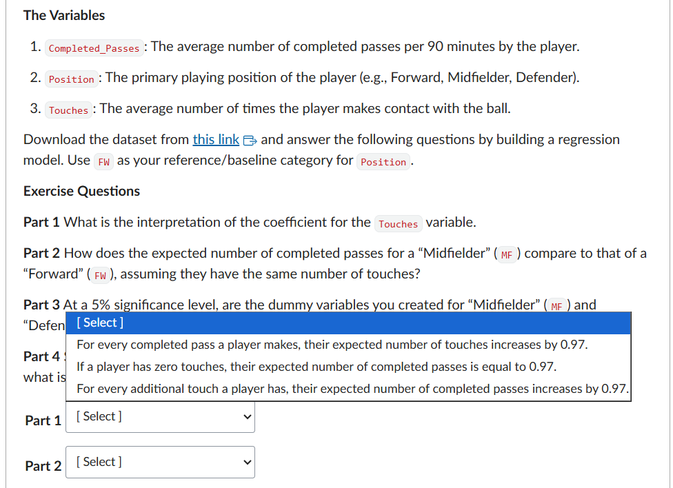
**The Variables**
1. `Completed_Passes`: The average number of completed passes per 90 minutes by the player.
2. `Position`: The primary playing position of the player (e.g., Forward, Midfielder, Defender).
3. `Touches`: The average number of times the player makes contact with the ball.
Download the dataset from [this link](`r download_url`) and answer the following questions by
building a regression model. Use `FW` as your reference/baseline category for `Position`.
**Exercise Questions**
**Part 1** What is the interpretation of the coefficient for the `Touches` variable.
**Part 2** How does the expected number of completed passes for a "Midfielder" (`MF`) compare to
that of a "Forward" (`FW`), assuming they have the same number of touches?
**Part 3** At a 5% significance level, are the dummy variables you created for "Midfielder" (`MF`)
and "Defender" (`DF`) statistically significant predictors?
**Part 4** San Diego FC is scouting a Midfielder who averages 90 touches per game. Using your
model, what is your prediction for his expected number of completed passes?
| Part | Answer Selection |
|:-----------|:-----------------|
| **Part 1** | ##ANSWER1## |
| **Part 2** | ##ANSWER2## |
| **Part 3** | ##ANSWER3## |
| **Part 4** | ##ANSWER4## |
```{r questionlist, echo = FALSE, results = "asis"}
answerlist(unlist(mget(paste0("part", 1:length(sols)), inherits = T)),
markup = "markdown")
```
The Compilation Pipeline
With the question templates ready, the compile.Rmd script orchestrates the final delivery. This process moves your code from a local environment to a live Canvas quiz.
Step 1: Authentication and Course Discovery
Before you can interact with Canvas, you must authenticate and identify the specific course where the quiz will be hosted.
library(exams)
library(vvcanvas)
library(data.table)

# 1. Authenticate with your Canvas API Token
canvas <- canvas_authenticate(token = "YOUR_TOKEN", url = "https://your-school.instructure.com")

# 2. Programmatically find your Course ID
# This avoids manual lookups in the browser
my_courses <- get_courses(canvas) |> data.table()
course_id <- my_courses[name %like% "Business Analytics", id]
Step 2: Generating the Randomized Package
Next, we use the exams2canvas function. This compiles your .Rmd templates into the QTI 1.2 format, generating as many unique variations as you specify.
# Bundling multiple question templates (Q1 and Q2) into a single quiz
# n = 50 ensures each student gets one of 50 unique versions
exams2canvas(c("Q1.Rmd", "soccer_scouting.Rmd"),
             n = 50,
             name = "Individual_Assignment_2")
Step 3: API Upload and Migration
Using the vvcanvas package, we push the generated .zip file directly to Canvas. The function returns a quiz_id, which we will use for the final configuration.
# This returns the ID of the newly created quiz shell
quiz_id <- upload_qti_file_with_migration(canvas, course_id, "Individual_Assignment_2.zip")
Step 4: Automating Quiz Metadata
Finally, we refine the quiz parameters. This step allows you to set the official title, provide clear HTML-formatted instructions, and control the publishing status.
# Refine the quiz settings directly from R
update_quiz(canvas, course_id, quiz_id, quiz_params = list(
  title = "Individual Assignment 2: European Scouting Challenge",
  description = "<h3>Instructions</h3>
    <p>Please download the dataset provided for each question
    and use Excel/R to complete your work.</p>
    <p><strong>Reminder:</strong> Every student receives a unique dataset.
    Your correct answers will be unique to your data.</p>",
  published = FALSE # Keep it hidden until you are ready
))
Conclusion
By separating the Question Design from the Compilation Logic, you create a modular system that can scale from a single quiz to an entire semester’s worth of automated assessments. The result is a high-integrity, professional environment where every student is challenged by a truly unique problem.